#data cleaning and preparationchess <- fide_ratings_september |>filter(!is.na(bday), !is.na(rating)) |>mutate(age =as.numeric(2026- bday)) |>group_by(age) |>summarise(avg_rating =mean(rating, na.rm =TRUE),n =n(),.groups ="drop" ) |>filter(n >=100) |>#filter so it isn't noisyarrange(age)
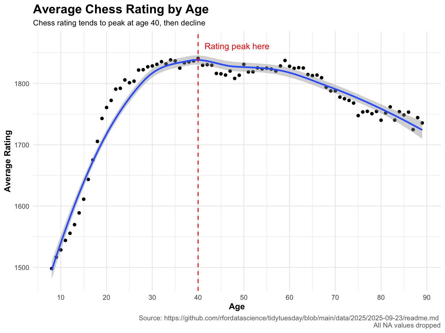
#Research question: How does age affect rating? For this data analysis, we took 200 thousand chess players from the FIDE tournament, and determined at what age rating tends to peak among these players.
Code
#Final visualizationggplot(chess, aes(x = age, y = avg_rating)) +geom_point() +labs(x ="Age", y ="Average Rating",title ="Average Chess Rating by Age",subtitle ="Chess rating tends to peak at age 40, then decline",caption ="Source: https://github.com/rfordatascience/tidytuesday/blob/main/data/2025/2025-09-23/readme.md \nAll NA values dropped") +scale_x_continuous(breaks =seq(0, 100, by =10)) +theme_minimal() +geom_smooth() +theme(plot.title =element_text(face ="bold", size =16),plot.subtitle =element_text(size =10),axis.title =element_text(face ="bold", size =11),plot.caption =element_text(color ="gray40") ) +geom_vline(xintercept =40,color ="red",linewidth =0.6,linetype ="dashed") +annotate("text",x =40,y =max(chess$avg_rating) +25,label ="Rating peak here",color ="red",hjust =-0.1,vjust =1)
Source Code
---title: "TidyTuesday2025-Week38"---```{r}#packageslibrary(tidyr)library(dplyr)library(ggplot2)#datafide_ratings_august <- readr::read_csv('https://raw.githubusercontent.com/rfordatascience/tidytuesday/main/data/2025/2025-09-23/fide_ratings_august.csv')fide_ratings_september <- readr::read_csv('https://raw.githubusercontent.com/rfordatascience/tidytuesday/main/data/2025/2025-09-23/fide_ratings_september.csv')``````{r}#data cleaning and preparationchess <- fide_ratings_september |>filter(!is.na(bday), !is.na(rating)) |>mutate(age =as.numeric(2026- bday)) |>group_by(age) |>summarise(avg_rating =mean(rating, na.rm =TRUE),n =n(),.groups ="drop" ) |>filter(n >=100) |>#filter so it isn't noisyarrange(age)```#Research question: How does age affect rating?For this data analysis, we took 200 thousand chess players from the FIDE tournament, and determined at what age rating tends to peak among these players.```{r, fig.width=8, fig.height=6}#Final visualizationggplot(chess, aes(x = age, y = avg_rating)) + geom_point() + labs(x = "Age", y = "Average Rating", title = "Average Chess Rating by Age", subtitle = "Chess rating tends to peak at age 40, then decline", caption = "Source: https://github.com/rfordatascience/tidytuesday/blob/main/data/2025/2025-09-23/readme.md \nAll NA values dropped") + scale_x_continuous(breaks = seq(0, 100, by = 10)) + theme_minimal() + geom_smooth() + theme( plot.title = element_text(face = "bold", size = 16), plot.subtitle = element_text(size = 10), axis.title = element_text(face = "bold", size = 11), plot.caption = element_text(color = "gray40") ) + geom_vline( xintercept = 40, color = "red", linewidth = 0.6, linetype = "dashed") + annotate( "text", x = 40, y = max(chess$avg_rating) + 25, label = "Rating peak here", color = "red", hjust = -0.1, vjust = 1)```