Homework 01
TidyTuesday Section
About the Data
The Tidy Tuesday data for the week of 9/2/25 comes from the sixth annual release of FrogID data. FrogID is a mobile app that enables citizen scientists in Australia to record and submit frog calls for experts to identify. Some key information provided in the dataset includes the time and location of the observation and taxonomic variables.
Driving Question: How do the observed numbers of different types of frogs vary temporally and spatially?
Temporal Analysis
First, I was interested in exploring how the abundances of different types of frogs, specifically tribes, vary over the course of a day. Are some tribes more active at night? In the afternoon?
To investigate my question, I created a new variable for the time of day. I mutated the event time variable, which is recorded in seconds, and divided it into four categories. “Night” includes 12 AM to 6 AM, “Morning” includes 6 AM to 12 PM, “Afternoon” includes 12 PM to 6 PM, and “Evening” includes 6 PM to 12 AM.
Code
# Create variable for categorizing the time
frog <- frog %>%
  mutate(
    time_of_day = case_when(
      eventTime >= 0 & eventTime < 21600 ~ "Night",
      eventTime >= 21600 & eventTime < 43200 ~ "Morning",
      eventTime >= 43200 & eventTime < 64800 ~ "Afternoon",
      eventTime >= 64800 & eventTime <= 86400 ~ "Evening"
))A mosaic plot was originally created for this assignment, but it no longer renders. The code was commented out and a proportional bar plot using the same variables was created.
Given that I am considering two categorical variables, time of day and tribe, I chose to visualize the data as a mosaic plot. The width of the columns is proportional to the number of observations at each time of day, and the vertical length of the bars is proportional to the number of observations for each tribe.
Code
# Remove entries where tribe is unknown
frog_plot <- frog %>%
  select(time_of_day, tribe) %>%
  na.omit() %>%
  mutate(
    time_of_day = fct_relevel(
      time_of_day, "Morning", "Afternoon", "Evening", "Night"
    )
  )

# Create mosaic plot
# ggplot(data = frog_plot %>% mutate(tribe = as.factor(tribe))) +
#  geom_mosaic(aes(x = product(time_of_day), fill = tribe)) +
#  theme(axis.text.y = element_blank(), axis.ticks.y = element_blank(),
#  axis.ticks.x = element_blank(), panel.background = element_blank(),
#  panel.grid.major = element_blank(), panel.grid.minor = element_blank()) +
#  labs(
#    title = "Australian Frog Tribe Abundances at Different Times of Day",
#    subtitle = "2023 FrogID Data", x = "Time of Day", y = "Tribe",
#  fill = "Tribe", caption = "Cate Stacy, 9/7/25, TidyTuesday")

ggplot(data = frog_plot) +
  geom_bar(aes(x = time_of_day, fill = tribe), position = "fill") +
  theme(axis.text.y = element_blank(), axis.ticks.y = element_blank(),
  axis.ticks.x = element_blank(), panel.background = element_blank(),
  panel.grid.major = element_blank(), panel.grid.minor = element_blank()) +
  labs(
    title = "Australian Frog Tribe Abundances at Different Times of Day", x = "", y = "",
    fill = "Tribe", caption = "Cate Stacy, 9/7/25, TidyTuesday 2023 FrogID Data")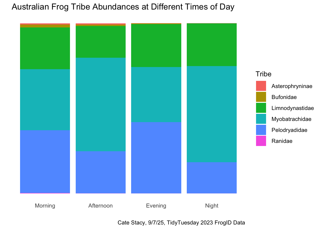
This plot shows that frogs are more abundant in the mornings and evenings, which include dawn and dusk. However, it should be noted that this trend could also reflect the behavior patterns of citizen scientists. For example, it makes sense that there would be fewer people making observations at night between the hours of 12 AM and 6 AM. The Pelodryadidae, Myobatrachidae, and Limnodynastidae tribes are far more abundant than the Asterophryninae, Bufonidae, and Ranidae tribes across all times of day. The Myobatrachidae tribe appears to be relatively more active at afternoon and night than in evening and morning. The Bufonidae tribe appears to be most active in the morning.
Spatial Analysis
I was also curious if the abundances of different frog tribes varies by region. I chose to visualize the relationship between state province and tribe as a balloon plot. The size of the circles corresponds to the number of frogs of a specific tribe in a given province.
Code
# Create new data frame in proper format for balloon plot
frog_plot2 <- frog %>%
  group_by(stateProvince, tribe) %>%
  summarize(Count = n()) %>%
  na.omit()

# Create balloon plot
ggballoonplot(frog_plot2, x = "stateProvince", y = "tribe",
  size = "Count", fill = "darkGreen") +
  labs(title = "Australian Frog Tribe Abundances Across State Provinces",
  subtitle = "2023 FrogID Data", y = "Tribe", x = "State Province",
  caption = "Cate Stacy, 9/7/25, TidyTuesday")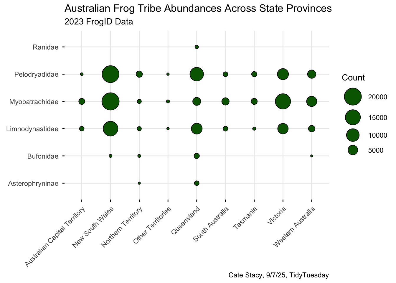
The plot demonstrates that New South Wales, Queensland, and Victoria had the most observations. However, it should be considered that there are potential confounding variables, including the size of the provinces and number of citizen scientists. This plot affirms the trend of Pelodryadidae, Myobatrachidae, and Limnodynastidae being most abundant, which was observed in the mosaic plot. An interesting finding is that the Ranidae tribe was only observed in Queensland. Additionally, despite having a relatively low total number of frogs, the Northern Territory had the second highest species richness (number of different species) and the highest species evenness (balanced relative abundance of different species).
Conclusions
Through creating visualizations, I was able to explore temporal and spatial variations in frog tribe abundance. More rigorous statistical analysis is required in order to make statements about the significance of the observed trends and account for potential confounding variables. However, the plots suggest that there are differences in frog activity among tribes and that the diversity and abundance of frogs varies across provinces.