12 Loops+Iter P2

library(purrr)
library(tidyverse)

🧩 Learning Goals

By the end of this lesson, you should be able to:

• Use the map() family of functions in the purrr package to handle repeated tasks that create output, instead of for loops
• Use the walk() family of functions in the purrr package to handle repeated tasks that need side-effects, instead of for loops

Iteration review

Let’s write a for loop that stores the class() (type) of every column in the mtcars data frame.

Yes, str() does this plus more for you. Let’s consider replicating this task through low-level iteration.

Recall that:

• vector("numeric/logical/character/list", length) creates a storage container.

• mtcars[[1]] accesses the first element/column of the data frame.

• First, write out the steps in words.

go over each column get the class of each column store the classes

• Then translate each step to code.

mtcars_vector <- vector("character", c(ncol(mtcars)))

for (i in seq_along(mtcars)) {
  mtcars_vector[i] <- class(mtcars[[i]])
}

mtcars_vector

 [1] "numeric" "numeric" "numeric" "numeric" "numeric" "numeric" "numeric"
 [8] "numeric" "numeric" "numeric" "numeric"

Iteration with purrr

purrr is a tidyverse package that provides several useful functions for iteration.

Open up the purrr cheatsheet.

The main advantages of purrr include:

• Improved readability of R code
• Reduction in the “overhead” in writing a for loop
  • These functions create storage containers
  • These functions do the for (i in ...) efficiently

Computational Time and Memory Allocation

Compare the four ways to create a vector of integers from 1 to 100,000.

# Example 1: For loop with no storage container; append new value to existing vector
x <- integer()
results1 <- bench::mark(
  for (i in 1:1e5) {
    x <- c(x, i)
  }
)

# Example 2: For loop with a storage container!
x <- vector('integer', length = 1e5)
results2 <- bench::mark(
  for (i in 1:1e5) {
    x[i] <- i
  }
)

# Example 3: purrr::map()
results3 <- bench::mark(purrr::map_int(1:1e5, ~.x))


# Example 4: Standard R Function/Operator
results4 <- bench::mark(seq(1,1e5))

# Compile Results
bind_rows(results1, results2, results3, results4) |>
  mutate(type = c("for_loop_no_storage", "for_loop_with_storage", "purrr_map", "standard_func")) |>
  select(type, mem_alloc, total_time)  |> print()

Iteration with map

In purrr, we can use the family of map() functions to iteratively apply a function to each element of a list or vector and save its output.

• Reminder: Data frames/tibbles are named lists so the elements are the “columns” so map() can iterate over columns of a dataset.

Let’s look at the purrr cheatsheet to look at graphical representations of how these functions work.

• map() returns a list
• map_chr() returns a character vector
• map_lgl() returns a logical vector
• map_int() returns an integer vector
• map_dbl() returns a numeric vector
• map_vec() returns a vector of a different (non-atomic) type (like dates)

Let’s return to our original task to replicate str().

To get the class() of each data frame column, map_chr() is sensible because classes are strings:

map_chr(mtcars, class)

      mpg       cyl      disp        hp      drat        wt      qsec        vs 
"numeric" "numeric" "numeric" "numeric" "numeric" "numeric" "numeric" "numeric" 
       am      gear      carb 
"numeric" "numeric" "numeric" 

Let’s get the class of each variable in diamonds:

map_chr(diamonds, class)

What happened!?

map_chr() was expecting to create a character vector with one element per element (column) in diamonds. But something happened in column 2 with the cut variable.

Let’s figure out what happened:

class(diamonds$cut)

[1] "ordered" "factor" 

Ah! cut has 2 classes. In this case, map() (which returns a list) is the best option because some variables have multiple classes:

map(diamonds, class)

$carat
[1] "numeric"

$cut
[1] "ordered" "factor" 

$color
[1] "ordered" "factor" 

$clarity
[1] "ordered" "factor" 

$depth
[1] "numeric"

$table
[1] "numeric"

$price
[1] "integer"

$x
[1] "numeric"

$y
[1] "numeric"

$z
[1] "numeric"

The error we encountered with map_chr() is a nice feature of purrr because it allows us to be very sure of the type of output we are getting.

Failing loudly is vastly preferable to getting unexpected outputs silently

Recall that we explored syntax and functions for selecting variables in a data frame via the tidy-select documentation for across. (?dplyr_tidy_select in the Console.)

We can also combine map_*() functions with tidy selection for some powerful variable summaries that require much less code than for loops.

# Mean of each numeric variable
map_dbl(diamonds |> select(where(is.numeric)), mean)

       carat        depth        table        price            x            y 
   0.7979397   61.7494049   57.4571839 3932.7997219    5.7311572    5.7345260 
           z 
   3.5387338 

# Number of unique values in each non-numeric variable
map_int(diamonds |> select(!where(is.numeric)), n_distinct)

    cut   color clarity 
      5       7       8 

Exercises

1. We want to compute several summary statistics on each quantitative variable in a data frame and organize the results in a new data frame (rows = variables, columns = summary statistics).

• Write a function called summ_stats() that takes a numeric vector x as input and returns the mean, median, standard deviation, and IQR as a data frame. You can use tibble() to create the data frame.
  • Example: tibble(a = 1:2, b = 2:3) creates a data frame with variables a and b.

diamonds_num <- diamonds |> select(where(is.numeric))

summ_stats <- function(x) {
  tibble(
    Mean = mean(x, na.rm = TRUE),
    Median = median(x, na.rm = TRUE),
    SD = sd(x, na.rm = TRUE),
    IQR = IQR(x, na.rm = TRUE)
  )
}

• Use a map*() function from purrr to get the summary statistics for each quantitative variable in diamonds.
• Look up the bind_rows() documentation from dplyr to combine summary statistics for all quantitative variables into one data frame.
  • Note: You’ll notice that the variable names are not present in the output. Try to figure out a way to add variable names back in with mutate() and colnames().

map(diamonds_num, summ_stats) |> 
  bind_rows() |> 
  mutate(variable = colnames(diamonds_num))

# A tibble: 7 × 5
      Mean  Median       SD     IQR variable
     <dbl>   <dbl>    <dbl>   <dbl> <chr>   
1    0.798    0.7     0.474    0.64 carat   
2   61.7     61.8     1.43     1.5  depth   
3   57.5     57       2.23     3    table   
4 3933.    2401    3989.    4374.   price   
5    5.73     5.7     1.12     1.83 x       
6    5.73     5.71    1.14     1.82 y       
7    3.54     3.53    0.706    1.13 z       

Once you’ve done that with map(), write a for loop to achieve the same result. Which do you prefer in terms of ease of code writing and readability?

diamond_summ_stats <- vector("list", length = ncol(diamonds_num))

for (i in seq_along(diamonds_num)) {
  diamond_summ_stats[[i]] <- summ_stats(diamonds_num[[i]])
} 
 
diamond_summ_stats |> 
  set_names(colnames(diamonds_num)) |> 
  bind_rows(.id = "variable")  

# A tibble: 7 × 5
  variable     Mean  Median       SD     IQR
  <chr>       <dbl>   <dbl>    <dbl>   <dbl>
1 carat       0.798    0.7     0.474    0.64
2 depth      61.7     61.8     1.43     1.5 
3 table      57.5     57       2.23     3   
4 price    3933.    2401    3989.    4374.  
5 x           5.73     5.7     1.12     1.83
6 y           5.73     5.71    1.14     1.82
7 z           3.54     3.53    0.706    1.13

Iteration with map2 or pmap

If you need to iterate over the rows of a data frame, we’ll need other versions of map().

purrr also offers map2() and the pmap() family of functions that take multiple inputs and loops over them simultaneously.

Let’s look at the purrr cheatsheet to look at graphical representations of how these functions work.

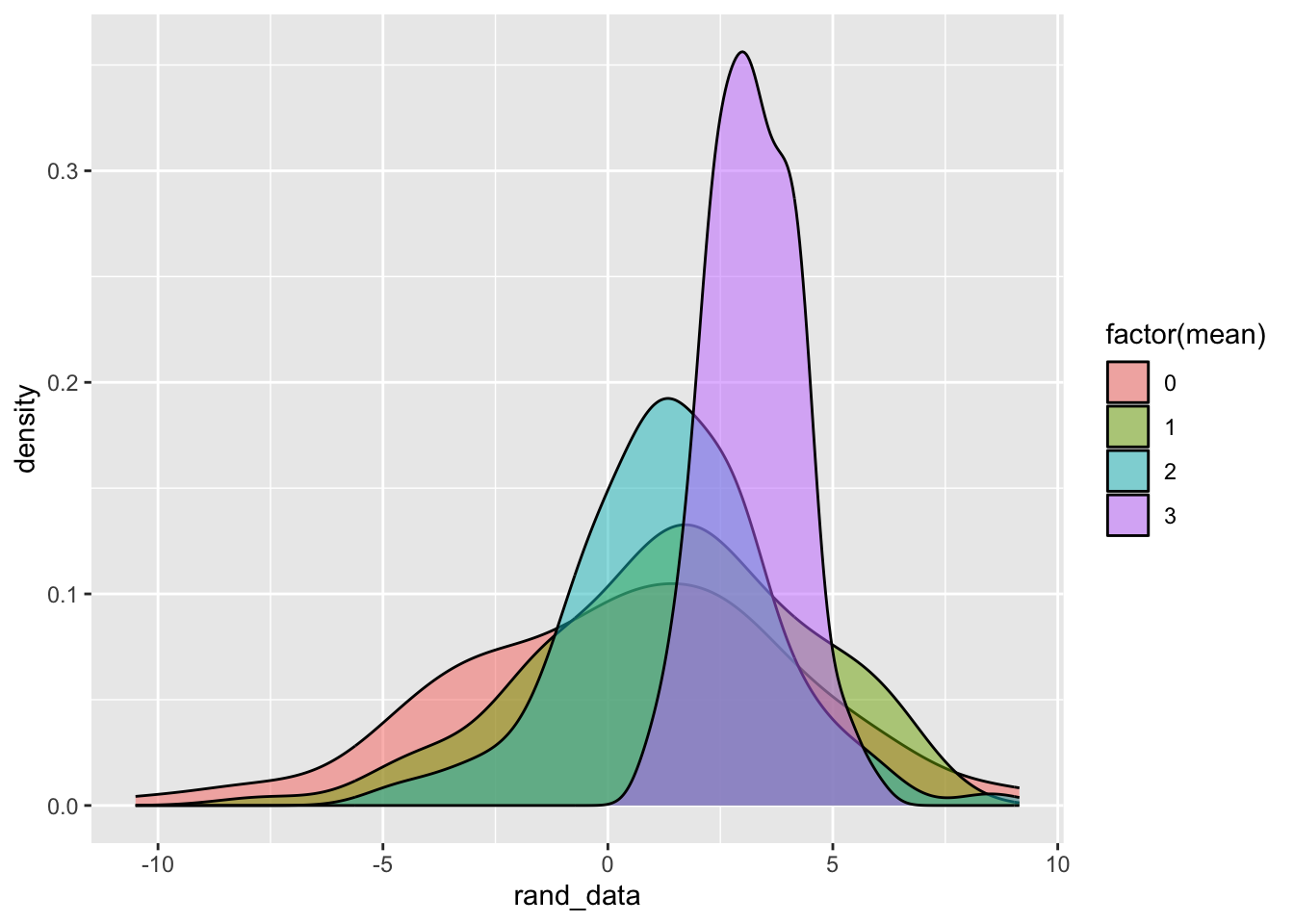
Let’s look at this code to randomly simulate data from Normal distributions.

args <- tibble(
  n = c(100, 100, 100, 100), # this is n
  mean = c(0, 1, 2, 3),            # this is mean
  sd = c(4, 3, 2, 1)            # this is sd
)

# save randomly generated data in tibble with simulation parameters
sim_data <- args |>
  mutate(rand_data = pmap(args, rnorm))

sim_data

# A tibble: 4 × 4
      n  mean    sd rand_data  
  <dbl> <dbl> <dbl> <list>     
1   100     0     4 <dbl [100]>
2   100     1     3 <dbl [100]>
3   100     2     2 <dbl [100]>
4   100     3     1 <dbl [100]>

Note how the column names in args exactly match the argument names in rnorm().

The iteration that is happening is across rows, and the multiple arguments in rnorm() are being matched by name.

To access the information in that rand_data list, we need to unnest() this list! It converts/unfolds the information into a numeric vector (repeating the information in mean, sd, n)

unnested_sim <- sim_data |> 
  unnest(rand_data) # convert the rand_data list to numeric vector
  
  
unnested_sim |> 
  ggplot(aes(x = rand_data, group = mean, fill = factor(mean))) +
  geom_density(alpha = .5)

We can also use pmap() to specify variations in some arguments but leave some arguments constant across the iterations:

string_data <- tibble(
    pattern = c("p", "n", "h"),
    replacement = c("P", "N", "H")
)

pmap_chr(string_data, str_replace_all, string = "ppp nnn hhh")

[1] "PPP nnn hhh" "ppp NNN hhh" "ppp nnn HHH"

Exercises

1. Create 2 small examples that show how pmap() works with str_sub(). Your examples should:

• Use different arguments for string, start, and end
• Use different arguments for start and end but a fixed string

string_data2 <- tibble(
  string = c("eye", "leg", "feet", "hands"),
  start = c(1, 2, 3, 2),
  end = c(1, 5, 4, 9)
)

pmap_chr(string_data2, str_sub)

[1] "e"    "eg"   "et"   "ands"

string_data3 <- tibble(
  start = c(1, 3, 5),
  end = c(1, 5, 10)
)

pmap_chr(string_data3, str_sub, string = "Hello World")

[1] "H"      "llo"    "o Worl"

2. Last class we worked on an extended exercise where our goal was to write a series of functions and a for loop to repeat linear model fitting under different “settings” (removal of outliers, model formula choice).

Repeat this exercise using pmap().

• You’ll need to use the df_arg_combos object, your remove_outliers() function, and your fit_model() function.
• Review the solutions below for the necessary parts and make sure you understand each part.
• Then, try to put it all together using pmap().

xs <- diamonds |> select(carat, cut, clarity, color) |> names()


df_arg_combos <- crossing(
    mod_formula = str_c("price ~ ", map_chr(seq_along(xs), ~ str_c(xs[1:.x], collapse = " + ")) ),
    remove_outliers = c(TRUE, FALSE)
)
df_arg_combos

# A tibble: 8 × 2
  mod_formula                           remove_outliers
  <chr>                                 <lgl>          
1 price ~ carat                         FALSE          
2 price ~ carat                         TRUE           
3 price ~ carat + cut                   FALSE          
4 price ~ carat + cut                   TRUE           
5 price ~ carat + cut + clarity         FALSE          
6 price ~ carat + cut + clarity         TRUE           
7 price ~ carat + cut + clarity + color FALSE          
8 price ~ carat + cut + clarity + color TRUE           

remove_outliers <- function(data, what_var, sd_thresh) {
    data |> 
        mutate(zscore = ({{ what_var }} - mean({{ what_var }}, na.rm = TRUE))/sd({{ what_var }}, na.rm = TRUE)) |>
        filter(zscore <= sd_thresh)
}

fit_model <- function(data, mod_formula, remove_outliers) {
    if (remove_outliers) {
        data_clean <- remove_outliers(data, what_var = carat, sd_thresh = 3)
    } else {
        data_clean <- data
    }
    
    lm(mod_formula, data = data_clean)
}

# use pmap()

df_arg_combos |> 
  mutate(fit_mod = pmap(df_arg_combos, fit_model, data = diamonds))

# A tibble: 8 × 3
  mod_formula                           remove_outliers fit_mod
  <chr>                                 <lgl>           <list> 
1 price ~ carat                         FALSE           <lm>   
2 price ~ carat                         TRUE            <lm>   
3 price ~ carat + cut                   FALSE           <lm>   
4 price ~ carat + cut                   TRUE            <lm>   
5 price ~ carat + cut + clarity         FALSE           <lm>   
6 price ~ carat + cut + clarity         TRUE            <lm>   
7 price ~ carat + cut + clarity + color FALSE           <lm>   
8 price ~ carat + cut + clarity + color TRUE            <lm>   

Iteration with walk

If we don’t care about saving an output for each iteration, we can use the family of walk() functions (walk, walk2, and pwalk) to apply a function to each element of a list or vector with no output.

Let’s say, we wanted to visualize the relationship between carat and price by clarity.

If we wanted a fully stratified (fully separated) analysis, we could create one visualization per clarity category and save it separately.

First, let’s create separate datasets that are still contained in one tibble.

# Let's create separate datasets within one tibble
by_clarity <- diamonds |> 
  group_nest(clarity)

by_clarity

# A tibble: 8 × 2
  clarity               data
  <ord>   <list<tibble[,9]>>
1 I1               [741 × 9]
2 SI2            [9,194 × 9]
3 SI1           [13,065 × 9]
4 VS2           [12,258 × 9]
5 VS1            [8,171 × 9]
6 VVS2           [5,066 × 9]
7 VVS1           [3,655 × 9]
8 IF             [1,790 × 9]

# Create a variable with a image path
by_clarity <- by_clarity |> 
  mutate(path = str_glue("diamonds-{clarity}.png"))

by_clarity

# A tibble: 8 × 3
  clarity               data path             
  <ord>   <list<tibble[,9]>> <glue>           
1 I1               [741 × 9] diamonds-I1.png  
2 SI2            [9,194 × 9] diamonds-SI2.png 
3 SI1           [13,065 × 9] diamonds-SI1.png 
4 VS2           [12,258 × 9] diamonds-VS2.png 
5 VS1            [8,171 × 9] diamonds-VS1.png 
6 VVS2           [5,066 × 9] diamonds-VVS2.png
7 VVS1           [3,655 × 9] diamonds-VVS1.png
8 IF             [1,790 × 9] diamonds-IF.png  

# plot for making a scatterplot
carat_scatter <- function(df) {
  ggplot(df, aes(x = carat, y = price)) + geom_point()  
}

# Create a "variable" with each plots
by_clarity <- by_clarity |> 
  mutate(plot = map(data, carat_scatter)) # iterate over data to create ggplot output

# Iterate over paths and plots to save the export images
walk2( 
  by_clarity$path,
  by_clarity$plot,
  function(path, plot){ ggsave(path, plot, width = 6, height = 6)}
)

Additional Resources

If you are interested in having a deeper understanding of the purrr package, I recommend you check out:

• Functionals Chapter in Advanced R by Hadley Wickham ## Done!

• Check the ICA Instructions for how to (a) push your code to GitHub and (b) update your portfolio website