TidyTuesday 09/02/2025

TidyTuesday Section

Explore the week’s TidyTuesday challenge. Develop a research question, then answer it through a short data story with effective visualization(s). Provide sufficient background for readers to grasp your narrative.

Code

#Necessary Libraries
#| include: false
#| echo: false

library(readxl)
library(dplyr)
library(tidyverse)
library(hrbrthemes)
library(viridis)

Importing Data

Reading in the data both about the families and genus of the frogs as well as individual frog ID events. The individual observation events were recorded frog calls by citizen scientists in Australia. The frogs were then identified via their calls by experts.

Code

Frog_ID <- read.csv("tidytuesday/data/2025/2025-09-02/frogID_data.csv")
Frog_names <- read.csv("tidytuesday/data/2025/2025-09-02/frog_names.csv")

Research Question: What subfamilies are the most abundant in Australia, and when are they the most abundant?

Exploring the Data

In order to create visualizations and have subfamilies corresponding to each observation I had to join the two different data sets by their scientific name.

Code

#Joining data sets together via scientific name and getting month of the observations
Frog_expanded <- 
  left_join(Frog_ID, Frog_names, by = "scientificName") |> 
  mutate(eventDate = as.Date(eventDate)) |> 
  mutate(month = format(eventDate, "%b"))

I then created a table that shows the counts of each subfamily of frog for each month over the year of 2023 in order to get an idea of what family was most abundant and when.

Code

#Demonstrating the count of each subfamily for each month
Frog_expanded |> 
  na.omit(subfamily) |> #omiting observations that do not have a subfamily, excludes >9000 observations
  count(month, subfamily) |> 
  mutate(month = factor(month, levels = month.abb, ordered = TRUE)) |> 
  arrange(month)

   month     subfamily     n
1    Jan         Hylid  8664
2    Jan  Microhylidae   155
3    Jan  Myobatrachid  7021
4    Jan         Ranid    12
5    Jan          Toad   282
6    Feb         Hylid  3675
7    Feb  Microhylidae   103
8    Feb  Myobatrachid  4735
9    Feb         Ranid     5
10   Feb          Toad   201
11   Mar         Hylid  1516
12   Mar  Microhylidae    53
13   Mar  Myobatrachid  4697
14   Mar         Ranid    15
15   Mar          Toad   112
16   Apr         Hylid   883
17   Apr  Microhylidae    21
18   Apr  Myobatrachid  5810
19   Apr         Ranid    22
20   Apr          Toad    36
21   May         Hylid   630
22   May  Microhylidae     7
23   May  Myobatrachid  3270
24   May         Ranid    13
25   May          Toad     9
26   Jun         Hylid  1291
27   Jun  Microhylidae    30
28   Jun  Myobatrachid  5002
29   Jun         Ranid    13
30   Jun          Toad    12
31   Jul         Hylid  1476
32   Jul  Microhylidae    60
33   Jul  Myobatrachid  7471
34   Jul         Ranid    21
35   Jul          Toad    36
36   Aug         Hylid  2634
37   Aug  Microhylidae    24
38   Aug  Myobatrachid 12016
39   Aug         Ranid    18
40   Aug          Toad    18
41   Sep         Hylid  5992
42   Sep  Microhylidae    48
43   Sep  Myobatrachid 12323
44   Sep         Ranid    12
45   Sep          Toad    74
46   Oct         Hylid  6851
47   Oct  Microhylidae    28
48   Oct  Myobatrachid  8677
49   Oct         Ranid    11
50   Oct          Toad    59
51   Nov         Hylid 11195
52   Nov  Microhylidae    38
53   Nov  Myobatrachid  9862
54   Nov         Ranid    19
55   Nov          Toad   209

It is important to note that in this case there are no observations for the month of December, so we cannot make a blanket statement saying the months Nov-Jan for example, as strickly speaking it is not true.

Visualizations

In order to get a better idea of the abundance of each family in comparison to the overall density for each month I created the following visualization.

Code

#Shows the overall amount of frogs over the year compared to the 
Frog_expanded |> 
  na.omit(subfamily) |>
  ggplot(aes(x = eventDate)) + 
  geom_density(aes(fill = subfamily), alpha = 0.5) +
  geom_histogram(aes(y = after_stat(density)), binwidth = 29, alpha = 0.5) + 
  theme_minimal() + 
  scale_fill_viridis_d() + 
  labs(x = "Date", y = "Density", title = "Density of Frogs and their Subfamilies over Time", subtitle = "2023", fill = "Subfamily")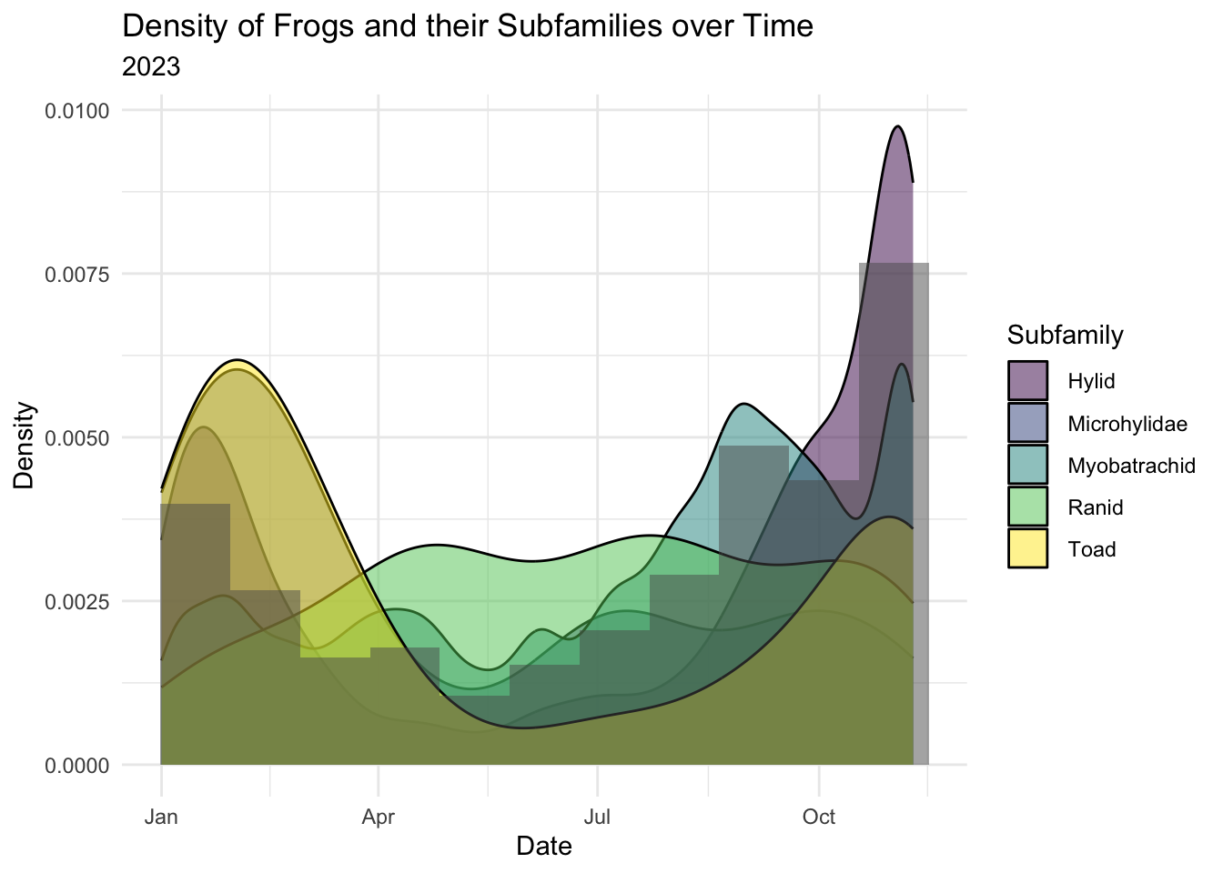

As we can see in above visualization is that frog calls tend to be more abundant October to January which is spring to summer in Australia. Toads most abundant around January-Febuary, late season. In comparison, Hylids are most abundant in December and January, mid to late season. Myobatrachid peaked in October as well as November. Ranid stay pretty consistent throughout the year. However the visuals layering of all the different subfamilies make it difficult to pull out exact measurements. For example, no trends for Microhylidae can be distinguished. The follow visualization splits all the different subfamiles so that they can be better compared against one another rather than the general trend.

Code

#Shows the distribution of each subfamily over the course of a year
Frog_expanded |> 
  na.omit(subfamily) |>
  ggplot(aes(x = eventDate, fill = subfamily)) +
  geom_density() +
  facet_wrap(~subfamily) + 
  labs(title = "Distribution of Subfamilies", subtitle = "2023", x = "Date", y = "Probability Density", fill = "Subfamily") + 
  theme_minimal() + 
  scale_fill_viridis_d()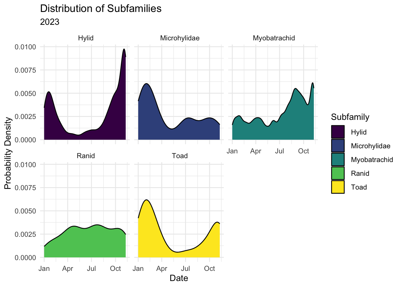

From this we can tell much more distinctly that Frogs that fall under the Microhylidae family tend to peak in January-Feburary while staying relatively consistent the rest of the year. However while this visual allows you to compare the density of each species relative to the total of each species not the total number of frogs or count. The following visualization addresses this issue.

Code

# Function to hide every other label
every_other_label <- function(x) {
      labels <- as.character(x)
      labels[seq(2, length(labels), 2)] <- ""
      return(labels)}

#Shows the proportion of the different frog families over the course of the year 
Frog_expanded |>
  na.omit(subfamily) |>
  mutate(month = factor(month, levels = month.abb, ordered = TRUE)) |> 
  ggplot(aes(x = month, , fill = subfamily)) + 
  geom_bar() + 
  facet_wrap(~subfamily) + 
  scale_fill_viridis_d() + 
  scale_x_discrete(labels = every_other_label) + 
  labs(x = "Month", y = "Number of Frogs", title = "The Number of Frogs of each Subfamily per Month", subtitle = "2023", fill = "Subfamily")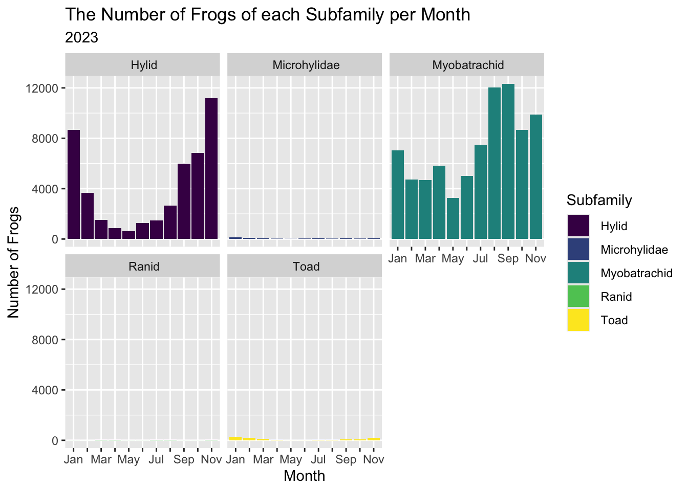

Through this visual we can clearly see that the Myobatrachid of frogs are the most abundant year round and make up most of the frogs that were documented in Australia in 2023. Hylids are the second most common subfamily, followed by Toad and Microhylidae and lastly Ranid. However because the last 3 categories are all significantly smaller than Hylids and Myobatrachid it is difficult to compare them.

Nevertheless we have answered the research question that Myobatrachids are the most abundant Frog subfamily in Australia and are more relatively abundant during the months of August to November.