6 Adv Data Wrangling P1

🧩 Learning Goals

By the end of this lesson, you should be able to:

  • Determine the class of a given object and identify concerns to be wary of when manipulating an object of that class (numerics, logicals, factors, dates, strings, data.frames)
  • Explain what vector recycling is, when it can be a problem, and how to avoid those problems
  • Use a variety of functions to wrangle numerical and logical data
  • Extract date-time information using the lubridate package
  • Use the forcats package to wrangle factor data

Helpful Cheatsheets

RStudio (Posit) maintains a collection of wonderful cheatsheets. The following will be helpful:

Data Wrangling Verbs (from Stat/Comp 112)

  • mutate(): creates/changes columns/elements in a data frame/tibble
  • select(): keeps subset of columns/elements in a data frame/tibble
  • filter(): keeps subsets of rows in a data frame/tibble
  • arrange(): sorts rows in a data frame/tibble
  • group_by(): internally groups rows in data frame/tibble by values in 1 or more columsn/elements
  • summarize(): collapses/combines information across rows using functions such as n(), sum(), mean(), min(), max(), median(), sd()
  • count(): shortcut for group_by() |> summarize(n = n())
  • left_join(): mutating join of two data frames/tibbles keeping all rows in left data frame
  • full_join(): mutating join of two data frames/tibbles keeping all rows in both data frames
  • inner_join(): mutating join of two data frames/tibbles keeping rows in left data frame that find match in right
  • semi_join(): filtering join of two data frames/tibbles keeping rows in left data frame that find match in right
  • anti_join(): filtering join of two data frames/tibbles keeping rows in left data frame that do not find match in right
  • pivot_wider(): rearrange values from two columns to many(one column becomes the names of new variables, one column becomes the values of the new variables)
  • pivot_longer(): rearrange values from many columns to two (the names of the columns go to one new variable, the values of the columns go to a second new variable)

Vectors

An atomic vector is a storage container in R where all elements in the container are of the same type. The types that are relevant to data science are:

  • logical (also known as boolean)
  • numbers
    • integer
    • numeric floating point (also known as double)
  • character string
  • Date and date-time (saved as POSIXct)
  • factor

Function documentation will refer to vectors frequently.

See examples below:

  • ggplot2::scale_x_continuous()
    • breaks: A numeric vector of positions
    • labels: A character vector giving labels (must be same length as breaks)
  • shiny::sliderInput()
    • value: The initial value of the slider […] A length one vector will create a regular slider; a length two vector will create a double-ended range slider.

When you need a vector, you can create one manually using

  • c(): the combine function

Or you can create one based on available data using

  • dataset |> mutate(newvar = variable > 5) |> pull(newvar): taking one column out of a dataset
  • dataset |> pull(variable) |> unique(): taking one column out of a dataset and finding unique values
Code
c("Fair", "Good", "Very Good", "Premium", "Ideal")
[1] "Fair"      "Good"      "Very Good" "Premium"   "Ideal"    
Code
diamonds |> pull(cut) |> unique()
[1] Ideal     Premium   Good      Very Good Fair     
Levels: Fair < Good < Very Good < Premium < Ideal

Logicals

Notes

What does a logical vector look like?

Code
x <- c(TRUE, FALSE, NA)
x
[1]  TRUE FALSE    NA
Code
class(x)
[1] "logical"

You will often create logical vectors with comparison operators: >, <, <=, >=, ==, !=.

Code
x <- c(1, 2, 9, 12)
x < 2
[1]  TRUE FALSE FALSE FALSE
Code
x <= 2
[1]  TRUE  TRUE FALSE FALSE
Code
x > 9
[1] FALSE FALSE FALSE  TRUE
Code
x >= 9
[1] FALSE FALSE  TRUE  TRUE
Code
x == 12
[1] FALSE FALSE FALSE  TRUE
Code
x != 12
[1]  TRUE  TRUE  TRUE FALSE

When you want to check for set containment, the %in% operator is the correct way to do this (as opposed to ==).

Code
x <- c(1, 2, 9, 4)
x == c(1, 2, 4)
Warning in x == c(1, 2, 4): longer object length is not a multiple of shorter
object length
[1]  TRUE  TRUE FALSE FALSE
Code
x %in% c(1, 2, 4)
[1]  TRUE  TRUE FALSE  TRUE

The Warning: longer object length is not a multiple of shorter object length is a manifestation of vector recycling.

In R, if two vectors are being combined or compared, the shorter one will be repeated to match the length of the longer one–even if longer object length isn’t a multiple of the shorter object length. We can see the exact recycling that happens below:

Code
x <- c(1, 2, 9, 4)
x == c(1, 2, 4)
[1]  TRUE  TRUE FALSE FALSE
Code
x == c(1, 2, 4, 1) # This line demonstrates the recycling that happens on the previous line
[1]  TRUE  TRUE FALSE FALSE

Logical vectors can also be created with functions. is.na() is one useful example:

Code
x <- c(1, 4, 9, NA)
x == NA
[1] NA NA NA NA
Code
is.na(x)
[1] FALSE FALSE FALSE  TRUE

We can negate a logical object with !. We can combine logical objects with & (and) and | (or).

Code
x <- c(1, 2, 4, 9)
x > 1 & x < 5
[1] FALSE  TRUE  TRUE FALSE
Code
!(x > 1 & x < 5)
[1]  TRUE FALSE FALSE  TRUE
Code
x < 2 | x > 8
[1]  TRUE FALSE FALSE  TRUE

We can summarize logical vectors with:

  • any(): Are ANY of the values TRUE?
  • all(): Are ALL of the values TRUE?
  • sum(): How many of the values are TRUE?
  • mean(): What fraction of the values are TRUE?
Code
x <- c(1, 2, 4, 9)
any(x == 1)
[1] TRUE
Code
all(x < 10)
[1] TRUE
Code
sum(x == 1)
[1] 1
Code
mean(x == 1)
[1] 0.25

if_else() and case_when() are functions that allow you to return values depending on the value of a logical vector. You’ll explore the documentation for these in the following exercises.

Note: ifelse() (from base R) and if_else() (from tidyverse) are different functions. We prefer if_else() for many reasons (examples below).

  • Noisy to make sure you catch issues/bugs
  • Can explicitly handle missing values
  • Keeps dates as dates
Examples
Code
x <- c(-1, -2, 4, 9, NA)

ifelse(x > 0, 'positive', 'negative')
[1] "negative" "negative" "positive" "positive" NA        
Code
if_else(x > 0, 'positive', 'negative')
[1] "negative" "negative" "positive" "positive" NA        
Code
ifelse(x > 0, 1, 'negative') # Bad: doesn't complain with combo of data types
[1] "negative" "negative" "1"        "1"        NA        
Code
if_else(x > 0, 1, 'negative') # Good:noisy to make sure you catch issues
Error in `if_else()`:
! Can't combine `true` <double> and `false` <character>.
Code
if_else(x > 0, 'positive', 'negative', missing = 'missing') # Good: can explicitly handle NA
[1] "negative" "negative" "positive" "positive" "missing" 
Code
fun_dates <- mdy('1-1-2025') + 0:365
ifelse(fun_dates < today(), fun_dates + years(), fun_dates) # Bad: converts dates to integers
  [1] 20454 20455 20456 20457 20458 20459 20460 20461 20462 20463 20464 20465
 [13] 20466 20467 20468 20469 20470 20471 20472 20473 20474 20475 20476 20477
 [25] 20478 20479 20480 20481 20482 20483 20484 20485 20486 20487 20488 20489
 [37] 20490 20491 20492 20493 20494 20495 20496 20497 20498 20499 20500 20501
 [49] 20502 20503 20504 20505 20506 20507 20508 20509 20510 20511 20512 20513
 [61] 20514 20515 20516 20517 20518 20519 20520 20521 20522 20523 20524 20525
 [73] 20526 20527 20528 20529 20530 20531 20532 20533 20534 20535 20536 20537
 [85] 20538 20539 20540 20541 20542 20543 20544 20545 20546 20547 20548 20549
 [97] 20550 20551 20552 20553 20554 20555 20556 20557 20558 20559 20560 20561
[109] 20562 20563 20564 20565 20566 20567 20568 20569 20570 20571 20572 20573
[121] 20574 20575 20576 20577 20578 20579 20580 20581 20582 20583 20584 20585
[133] 20586 20587 20588 20589 20590 20591 20592 20593 20594 20595 20596 20597
[145] 20598 20599 20600 20601 20602 20603 20604 20605 20606 20607 20608 20609
[157] 20610 20611 20612 20613 20614 20615 20616 20617 20618 20619 20620 20621
[169] 20622 20623 20624 20625 20626 20627 20628 20629 20630 20631 20632 20633
[181] 20634 20635 20636 20637 20638 20639 20640 20641 20642 20643 20644 20645
[193] 20646 20647 20648 20649 20650 20651 20652 20653 20654 20655 20656 20657
[205] 20658 20659 20660 20661 20662 20663 20664 20665 20666 20667 20668 20669
[217] 20670 20671 20672 20673 20674 20675 20676 20677 20678 20679 20680 20681
[229] 20682 20683 20684 20685 20686 20687 20688 20689 20690 20691 20692 20693
[241] 20694 20695 20696 20697 20698 20699 20700 20701 20702 20703 20704 20705
[253] 20706 20707 20708 20709 20710 20711 20712 20713 20714 20715 20716 20717
[265] 20718 20719 20720 20721 20722 20723 20724 20725 20726 20727 20728 20729
[277] 20730 20731 20732 20733 20734 20735 20736 20737 20738 20739 20740 20741
[289] 20742 20743 20744 20745 20381 20382 20383 20384 20385 20386 20387 20388
[301] 20389 20390 20391 20392 20393 20394 20395 20396 20397 20398 20399 20400
[313] 20401 20402 20403 20404 20405 20406 20407 20408 20409 20410 20411 20412
[325] 20413 20414 20415 20416 20417 20418 20419 20420 20421 20422 20423 20424
[337] 20425 20426 20427 20428 20429 20430 20431 20432 20433 20434 20435 20436
[349] 20437 20438 20439 20440 20441 20442 20443 20444 20445 20446 20447 20448
[361] 20449 20450 20451 20452 20453 20454
Code
if_else(fun_dates < today(), fun_dates + years(), fun_dates) # Good: keeps dates as dates
  [1] "2026-01-01" "2026-01-02" "2026-01-03" "2026-01-04" "2026-01-05"
  [6] "2026-01-06" "2026-01-07" "2026-01-08" "2026-01-09" "2026-01-10"
 [11] "2026-01-11" "2026-01-12" "2026-01-13" "2026-01-14" "2026-01-15"
 [16] "2026-01-16" "2026-01-17" "2026-01-18" "2026-01-19" "2026-01-20"
 [21] "2026-01-21" "2026-01-22" "2026-01-23" "2026-01-24" "2026-01-25"
 [26] "2026-01-26" "2026-01-27" "2026-01-28" "2026-01-29" "2026-01-30"
 [31] "2026-01-31" "2026-02-01" "2026-02-02" "2026-02-03" "2026-02-04"
 [36] "2026-02-05" "2026-02-06" "2026-02-07" "2026-02-08" "2026-02-09"
 [41] "2026-02-10" "2026-02-11" "2026-02-12" "2026-02-13" "2026-02-14"
 [46] "2026-02-15" "2026-02-16" "2026-02-17" "2026-02-18" "2026-02-19"
 [51] "2026-02-20" "2026-02-21" "2026-02-22" "2026-02-23" "2026-02-24"
 [56] "2026-02-25" "2026-02-26" "2026-02-27" "2026-02-28" "2026-03-01"
 [61] "2026-03-02" "2026-03-03" "2026-03-04" "2026-03-05" "2026-03-06"
 [66] "2026-03-07" "2026-03-08" "2026-03-09" "2026-03-10" "2026-03-11"
 [71] "2026-03-12" "2026-03-13" "2026-03-14" "2026-03-15" "2026-03-16"
 [76] "2026-03-17" "2026-03-18" "2026-03-19" "2026-03-20" "2026-03-21"
 [81] "2026-03-22" "2026-03-23" "2026-03-24" "2026-03-25" "2026-03-26"
 [86] "2026-03-27" "2026-03-28" "2026-03-29" "2026-03-30" "2026-03-31"
 [91] "2026-04-01" "2026-04-02" "2026-04-03" "2026-04-04" "2026-04-05"
 [96] "2026-04-06" "2026-04-07" "2026-04-08" "2026-04-09" "2026-04-10"
[101] "2026-04-11" "2026-04-12" "2026-04-13" "2026-04-14" "2026-04-15"
[106] "2026-04-16" "2026-04-17" "2026-04-18" "2026-04-19" "2026-04-20"
[111] "2026-04-21" "2026-04-22" "2026-04-23" "2026-04-24" "2026-04-25"
[116] "2026-04-26" "2026-04-27" "2026-04-28" "2026-04-29" "2026-04-30"
[121] "2026-05-01" "2026-05-02" "2026-05-03" "2026-05-04" "2026-05-05"
[126] "2026-05-06" "2026-05-07" "2026-05-08" "2026-05-09" "2026-05-10"
[131] "2026-05-11" "2026-05-12" "2026-05-13" "2026-05-14" "2026-05-15"
[136] "2026-05-16" "2026-05-17" "2026-05-18" "2026-05-19" "2026-05-20"
[141] "2026-05-21" "2026-05-22" "2026-05-23" "2026-05-24" "2026-05-25"
[146] "2026-05-26" "2026-05-27" "2026-05-28" "2026-05-29" "2026-05-30"
[151] "2026-05-31" "2026-06-01" "2026-06-02" "2026-06-03" "2026-06-04"
[156] "2026-06-05" "2026-06-06" "2026-06-07" "2026-06-08" "2026-06-09"
[161] "2026-06-10" "2026-06-11" "2026-06-12" "2026-06-13" "2026-06-14"
[166] "2026-06-15" "2026-06-16" "2026-06-17" "2026-06-18" "2026-06-19"
[171] "2026-06-20" "2026-06-21" "2026-06-22" "2026-06-23" "2026-06-24"
[176] "2026-06-25" "2026-06-26" "2026-06-27" "2026-06-28" "2026-06-29"
[181] "2026-06-30" "2026-07-01" "2026-07-02" "2026-07-03" "2026-07-04"
[186] "2026-07-05" "2026-07-06" "2026-07-07" "2026-07-08" "2026-07-09"
[191] "2026-07-10" "2026-07-11" "2026-07-12" "2026-07-13" "2026-07-14"
[196] "2026-07-15" "2026-07-16" "2026-07-17" "2026-07-18" "2026-07-19"
[201] "2026-07-20" "2026-07-21" "2026-07-22" "2026-07-23" "2026-07-24"
[206] "2026-07-25" "2026-07-26" "2026-07-27" "2026-07-28" "2026-07-29"
[211] "2026-07-30" "2026-07-31" "2026-08-01" "2026-08-02" "2026-08-03"
[216] "2026-08-04" "2026-08-05" "2026-08-06" "2026-08-07" "2026-08-08"
[221] "2026-08-09" "2026-08-10" "2026-08-11" "2026-08-12" "2026-08-13"
[226] "2026-08-14" "2026-08-15" "2026-08-16" "2026-08-17" "2026-08-18"
[231] "2026-08-19" "2026-08-20" "2026-08-21" "2026-08-22" "2026-08-23"
[236] "2026-08-24" "2026-08-25" "2026-08-26" "2026-08-27" "2026-08-28"
[241] "2026-08-29" "2026-08-30" "2026-08-31" "2026-09-01" "2026-09-02"
[246] "2026-09-03" "2026-09-04" "2026-09-05" "2026-09-06" "2026-09-07"
[251] "2026-09-08" "2026-09-09" "2026-09-10" "2026-09-11" "2026-09-12"
[256] "2026-09-13" "2026-09-14" "2026-09-15" "2026-09-16" "2026-09-17"
[261] "2026-09-18" "2026-09-19" "2026-09-20" "2026-09-21" "2026-09-22"
[266] "2026-09-23" "2026-09-24" "2026-09-25" "2026-09-26" "2026-09-27"
[271] "2026-09-28" "2026-09-29" "2026-09-30" "2026-10-01" "2026-10-02"
[276] "2026-10-03" "2026-10-04" "2026-10-05" "2026-10-06" "2026-10-07"
[281] "2026-10-08" "2026-10-09" "2026-10-10" "2026-10-11" "2026-10-12"
[286] "2026-10-13" "2026-10-14" "2026-10-15" "2026-10-16" "2026-10-17"
[291] "2026-10-18" "2026-10-19" "2025-10-20" "2025-10-21" "2025-10-22"
[296] "2025-10-23" "2025-10-24" "2025-10-25" "2025-10-26" "2025-10-27"
[301] "2025-10-28" "2025-10-29" "2025-10-30" "2025-10-31" "2025-11-01"
[306] "2025-11-02" "2025-11-03" "2025-11-04" "2025-11-05" "2025-11-06"
[311] "2025-11-07" "2025-11-08" "2025-11-09" "2025-11-10" "2025-11-11"
[316] "2025-11-12" "2025-11-13" "2025-11-14" "2025-11-15" "2025-11-16"
[321] "2025-11-17" "2025-11-18" "2025-11-19" "2025-11-20" "2025-11-21"
[326] "2025-11-22" "2025-11-23" "2025-11-24" "2025-11-25" "2025-11-26"
[331] "2025-11-27" "2025-11-28" "2025-11-29" "2025-11-30" "2025-12-01"
[336] "2025-12-02" "2025-12-03" "2025-12-04" "2025-12-05" "2025-12-06"
[341] "2025-12-07" "2025-12-08" "2025-12-09" "2025-12-10" "2025-12-11"
[346] "2025-12-12" "2025-12-13" "2025-12-14" "2025-12-15" "2025-12-16"
[351] "2025-12-17" "2025-12-18" "2025-12-19" "2025-12-20" "2025-12-21"
[356] "2025-12-22" "2025-12-23" "2025-12-24" "2025-12-25" "2025-12-26"
[361] "2025-12-27" "2025-12-28" "2025-12-29" "2025-12-30" "2025-12-31"
[366] "2026-01-01"

Exercises

Load the diamonds dataset, and filter to the first 1000 diamonds.

Code
data(diamonds)
diamonds <- diamonds |> 
    slice_head(n = 1000)

Using tidyverse functions, complete the following:

  1. Subset to diamonds that are less than 400 dollars or more than 10000 dollars.
  2. Subset to diamonds that are between 500 and 600 dollars (inclusive).
  3. How many diamonds are of either Fair, Premium, or Ideal cut (a total count)? What fraction of diamonds are of Fair, Premium, or Ideal cut?
    • First, do this a wrong way with ==. Predict the warning message that you will receive.
    • Second, do this the correct way with an appropriate logical operator.
  4. Are there any diamonds of Fair cut that are more than $3000? Are all diamonds of Ideal cut more than $2000?
  5. Create two new categorized versions of price by looking up the documentation for if_else() and case_when():
    • price_cat1: “low” if price is less than 500 and “high” otherwise
    • price_cat2: “low” if price is less than 500, “medium” if price is between 500 and 1000 dollars inclusive, and “high” otherwise.
Code
#1
diamonds |> 
  filter(price < 400 | price > 10000)
# A tibble: 30 × 10
   carat cut       color clarity depth table price     x     y     z
   <dbl> <ord>     <ord> <ord>   <dbl> <dbl> <int> <dbl> <dbl> <dbl>
 1  0.23 Ideal     E     SI2      61.5    55   326  3.95  3.98  2.43
 2  0.21 Premium   E     SI1      59.8    61   326  3.89  3.84  2.31
 3  0.23 Good      E     VS1      56.9    65   327  4.05  4.07  2.31
 4  0.29 Premium   I     VS2      62.4    58   334  4.2   4.23  2.63
 5  0.31 Good      J     SI2      63.3    58   335  4.34  4.35  2.75
 6  0.24 Very Good J     VVS2     62.8    57   336  3.94  3.96  2.48
 7  0.24 Very Good I     VVS1     62.3    57   336  3.95  3.98  2.47
 8  0.26 Very Good H     SI1      61.9    55   337  4.07  4.11  2.53
 9  0.22 Fair      E     VS2      65.1    61   337  3.87  3.78  2.49
10  0.23 Very Good H     VS1      59.4    61   338  4     4.05  2.39
# ℹ 20 more rows
Code
#2
diamonds |> 
  filter(price >= 500 & price <= 600)
# A tibble: 90 × 10
   carat cut       color clarity depth table price     x     y     z
   <dbl> <ord>     <ord> <ord>   <dbl> <dbl> <int> <dbl> <dbl> <dbl>
 1  0.35 Ideal     I     VS1      60.9  57     552  4.54  4.59  2.78
 2  0.3  Premium   D     SI1      62.6  59     552  4.23  4.27  2.66
 3  0.3  Ideal     D     SI1      62.5  57     552  4.29  4.32  2.69
 4  0.3  Ideal     D     SI1      62.1  56     552  4.3   4.33  2.68
 5  0.42 Premium   I     SI2      61.5  59     552  4.78  4.84  2.96
 6  0.28 Ideal     G     VVS2     61.4  56     553  4.19  4.22  2.58
 7  0.32 Ideal     I     VVS1     62    55.3   553  4.39  4.42  2.73
 8  0.31 Very Good G     SI1      63.3  57     553  4.33  4.3   2.73
 9  0.31 Premium   G     SI1      61.8  58     553  4.35  4.32  2.68
10  0.24 Premium   E     VVS1     60.7  58     553  4.01  4.03  2.44
# ℹ 80 more rows
Code
#3
diamonds |> 
  mutate(is_fpi = cut %in% c("Fair", "Premium", "Ideal")) |> 
  summarise(Total_fpi = sum(is_fpi), Frac_fpi = mean(is_fpi))
# A tibble: 1 × 2
  Total_fpi Frac_fpi
      <int>    <dbl>
1       685    0.685
Code
#4
diamonds |> 
  filter(cut == "Fair") |> 
  summarise(price_high = any(price > 3000))
# A tibble: 1 × 1
  price_high
  <lgl>     
1 FALSE     
Code
diamonds |> 
  filter(cut == "Ideal") |> 
  summarise(price_high = all(price > 2000))
# A tibble: 1 × 1
  price_high
  <lgl>     
1 FALSE     
Code
#5
diamonds |> 
  mutate(
  price_cat1 = if_else(price < 500, "low", "high"), 
  price_cat2 = case_when(
    price < 500 ~ "low",
    price >= 500 & price <= 1000 ~ "medium",
    price > 1000 ~ "high")
  )
# A tibble: 1,000 × 12
   carat cut       color clarity depth table price     x     y     z price_cat1
   <dbl> <ord>     <ord> <ord>   <dbl> <dbl> <int> <dbl> <dbl> <dbl> <chr>     
 1  0.23 Ideal     E     SI2      61.5    55   326  3.95  3.98  2.43 low       
 2  0.21 Premium   E     SI1      59.8    61   326  3.89  3.84  2.31 low       
 3  0.23 Good      E     VS1      56.9    65   327  4.05  4.07  2.31 low       
 4  0.29 Premium   I     VS2      62.4    58   334  4.2   4.23  2.63 low       
 5  0.31 Good      J     SI2      63.3    58   335  4.34  4.35  2.75 low       
 6  0.24 Very Good J     VVS2     62.8    57   336  3.94  3.96  2.48 low       
 7  0.24 Very Good I     VVS1     62.3    57   336  3.95  3.98  2.47 low       
 8  0.26 Very Good H     SI1      61.9    55   337  4.07  4.11  2.53 low       
 9  0.22 Fair      E     VS2      65.1    61   337  3.87  3.78  2.49 low       
10  0.23 Very Good H     VS1      59.4    61   338  4     4.05  2.39 low       
# ℹ 990 more rows
# ℹ 1 more variable: price_cat2 <chr>

Numerics

Notes

Numerical data can be of class integer or numeric (representing real numbers).

Code
x <- 1:3
x
[1] 1 2 3
Code
class(x)
[1] "integer"
Code
x <- c(1+1e-9, 2, 3)
x
[1] 1 2 3
Code
class(x)
[1] "numeric"

The Numbers chapter in R4DS covers the following functions that are all useful for wrangling numeric data:

  • n(), n_distinct(): Counting and counting the number of unique values
  • sum(is.na()): Counting the number of missing values
  • min(), max()
  • pmin(), pmax(): Get the min and max across several vectors
  • Integer division: %/%. Remainder: %%
    • 121 %/% 100 = 1 and 121 %% 100 = 21
  • round(), floor(), ceiling(): Rounding functions (to a specified number of decimal places, to the largest integer below a number, to the smallest integer above a number)
  • cut(): Cut a numerical vector into categories
  • cumsum(), cummean(), cummin(), cummax(): Cumulative functions
  • rank(): Provide the ranks of the numbers in a vector
  • lead(), lag(): shift a vector by padding with NAs
  • Numerical summaries: mean, median, min, max, quantile, sd, IQR
    • Note that all numerical summary functions have an na.rm argument that should be set to TRUE if you have missing data.

Exercises

Exercises will be on HW4.

The best way to add these functions and operators to your vocabulary is to need to recall them. Refer to the list of functions above as you try the exercises.

You will need to reference function documentation to look at arguments and look in the Examples section.

Dates

Notes

The lubridate package contains useful functions for working with dates and times. The lubridate function reference is a useful resource for finding the functions you need. We’ll take a brief tour of this reference page.

We’ll use the lakers dataset in the lubridate package to illustrate some examples.

Code
lakers <- as_tibble(lakers)
head(lakers)
# A tibble: 6 × 13
     date opponent game_type time  period etype team  player result points type 
    <int> <chr>    <chr>     <chr>  <int> <chr> <chr> <chr>  <chr>   <int> <chr>
1  2.01e7 POR      home      12:00      1 jump… OFF   ""     ""          0 ""   
2  2.01e7 POR      home      11:39      1 shot  LAL   "Pau … "miss…      0 "hoo…
3  2.01e7 POR      home      11:37      1 rebo… LAL   "Vlad… ""          0 "off"
4  2.01e7 POR      home      11:25      1 shot  LAL   "Dere… "miss…      0 "lay…
5  2.01e7 POR      home      11:23      1 rebo… LAL   "Pau … ""          0 "off"
6  2.01e7 POR      home      11:22      1 shot  LAL   "Pau … "made"      2 "hoo…
# ℹ 2 more variables: x <int>, y <int>

Below we use date-time parsing functions to represent the date and time variables with date-time classes:

Code
lakers <- lakers |>
    mutate(
        date = ymd(date),
        time = ms(time)
    )

Below we use extraction functions to get components of the date-time objects:

Code
lakers_clean <- lakers |>
    mutate(
        year = year(date),
        month = month(date),
        day = day(date),
        day_of_week = wday(date, label = TRUE),
        minute = minute(time),
        second = second(time)
    )
lakers_clean |> select(year:second)
# A tibble: 34,624 × 6
    year month   day day_of_week minute second
   <dbl> <dbl> <int> <ord>        <dbl>  <dbl>
 1  2008    10    28 Tue             12      0
 2  2008    10    28 Tue             11     39
 3  2008    10    28 Tue             11     37
 4  2008    10    28 Tue             11     25
 5  2008    10    28 Tue             11     23
 6  2008    10    28 Tue             11     22
 7  2008    10    28 Tue             11     22
 8  2008    10    28 Tue             11     22
 9  2008    10    28 Tue             11      0
10  2008    10    28 Tue             10     53
# ℹ 34,614 more rows
Code
lakers_clean <- lakers_clean |>
    group_by(date, opponent, period) |>
    arrange(date, opponent, period, desc(time)) |>
    mutate(
        diff_btw_plays_sec = as.numeric(time - lag(time, 1))
    )
lakers_clean |> select(date, opponent, time, period, diff_btw_plays_sec)
# A tibble: 34,624 × 5
# Groups:   date, opponent, period [314]
   date       opponent time     period diff_btw_plays_sec
   <date>     <chr>    <Period>  <int>              <dbl>
 1 2008-10-28 POR      12M 0S        1                 NA
 2 2008-10-28 POR      11M 39S       1                -21
 3 2008-10-28 POR      11M 37S       1                 -2
 4 2008-10-28 POR      11M 25S       1                -12
 5 2008-10-28 POR      11M 23S       1                 -2
 6 2008-10-28 POR      11M 22S       1                 -1
 7 2008-10-28 POR      11M 22S       1                  0
 8 2008-10-28 POR      11M 22S       1                  0
 9 2008-10-28 POR      11M 0S        1                -22
10 2008-10-28 POR      10M 53S       1                 -7
# ℹ 34,614 more rows

Exercises

Exercises will be on HW4.

Factors

Notes

Creating factors

In R, factors are made up of two components: the actual values of the data and the possible levels within the factor. Creating a factor requires supplying both pieces of information.

Code
months <- c("Mar", "Dec", "Jan",  "Apr", "Jul")

However, if we were to sort this vector, R would sort this vector alphabetically.

Code
# alphabetical sort
sort(months)
[1] "Apr" "Dec" "Jan" "Jul" "Mar"

We can fix this sorting by creating a factor version of months. The levels argument is a character vector that specifies the unique values that the factor can take. The order of the values in levels defines the sorting of the factor.

Code
months_fct <- factor(months, levels = month.abb) # month.abb is a built-in variable
months_fct
[1] Mar Dec Jan Apr Jul
Levels: Jan Feb Mar Apr May Jun Jul Aug Sep Oct Nov Dec
Code
sort(months_fct)
[1] Jan Mar Apr Jul Dec
Levels: Jan Feb Mar Apr May Jun Jul Aug Sep Oct Nov Dec

What if we try to create a factor with values that aren’t in the levels? (e.g., a typo in a month name)

Code
months2 <- c("Jna", "Mar")
factor(months2, levels = month.abb)
[1] <NA> Mar 
Levels: Jan Feb Mar Apr May Jun Jul Aug Sep Oct Nov Dec

Because the NA is introduced silently (without any error or warnings), this can be dangerous. It might be better to use the fct() function in the forcats package instead:

Code
fct(months2, levels = month.abb)
Error in `fct()`:
! All values of `x` must appear in `levels` or `na`
ℹ Missing level: "Jna"

Reordering factors

We’ll use a subset of the General Social Survey (GSS) dataset available in the forcats pacakges.

Code
data(gss_cat)
head(gss_cat)
# A tibble: 6 × 9
   year marital         age race  rincome        partyid     relig denom tvhours
  <int> <fct>         <int> <fct> <fct>          <fct>       <fct> <fct>   <int>
1  2000 Never married    26 White $8000 to 9999  Ind,near r… Prot… Sout…      12
2  2000 Divorced         48 White $8000 to 9999  Not str re… Prot… Bapt…      NA
3  2000 Widowed          67 White Not applicable Independent Prot… No d…       2
4  2000 Never married    39 White Not applicable Ind,near r… Orth… Not …       4
5  2000 Divorced         25 White Not applicable Not str de… None  Not …       1
6  2000 Married          25 White $20000 - 24999 Strong dem… Prot… Sout…      NA

Reordering the levels of a factor can be useful in plotting when categories would benefit from being sorted in a particular way:

Code
relig_summary <- gss_cat |>
    group_by(relig) |>
    summarize(
        tvhours = mean(tvhours, na.rm = TRUE),
        n = n()
    )

ggplot(relig_summary, aes(x = tvhours, y = relig)) + 
    geom_point() +
    theme_classic()

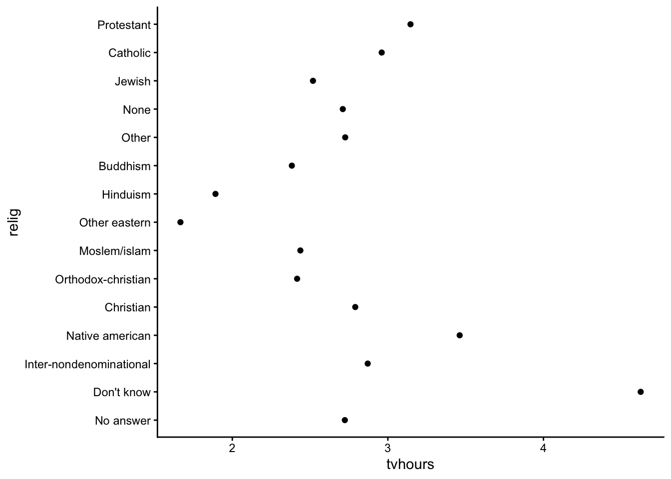
We can use fct_reorder() in forcats.

  • The first argument is the factor that you want to reorder the levels of
  • The second argument determines how the factor is sorted (analogous to what you put inside arrange() when sorting the rows of a data frame.)
Code
ggplot(relig_summary, aes(x = tvhours, y = fct_reorder(relig, tvhours))) +
    geom_point() +
    theme_classic()

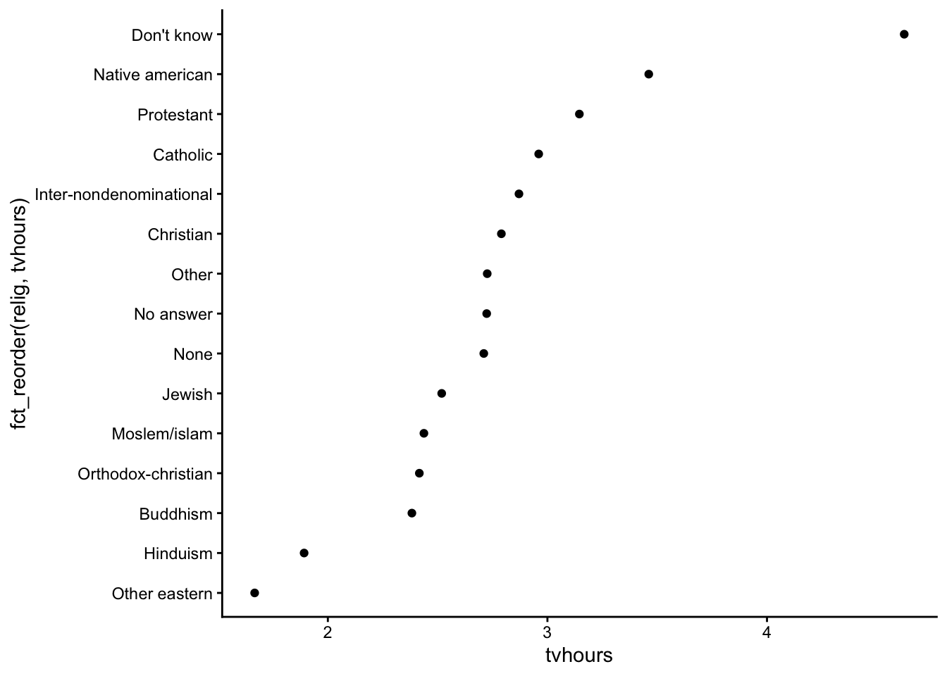
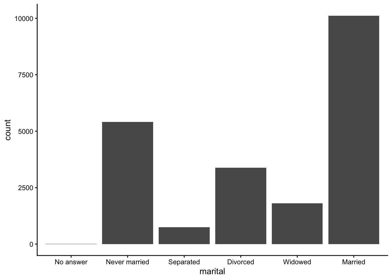
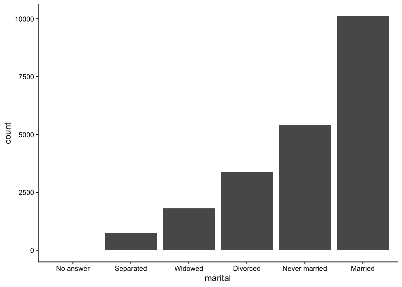
For bar plots, we can use fct_infreq() to reorder levels from most to least common. This can be combined with fct_rev() to reverse the order (least to most common):

Code
gss_cat |>
    ggplot(aes(x = marital)) +
    geom_bar() +
    theme_classic()

Code
gss_cat |>
    mutate(marital = marital |> fct_infreq() |> fct_rev()) |>
    ggplot(aes(x = marital)) +
    geom_bar() +
    theme_classic()

Modifying factor levels

We talked about reordering the levels of a factor–what about changing the values of the levels themselves?

For example, the names of the political parties in the GSS could use elaboration (“str” isn’t a great label for “strong”) and clean up:

Code
gss_cat |> count(partyid)
# A tibble: 10 × 2
   partyid                n
   <fct>              <int>
 1 No answer            154
 2 Don't know             1
 3 Other party          393
 4 Strong republican   2314
 5 Not str republican  3032
 6 Ind,near rep        1791
 7 Independent         4119
 8 Ind,near dem        2499
 9 Not str democrat    3690
10 Strong democrat     3490

We can use fct_recode() on partyid with the new level names going on the left and the old levels on the right. Any levels that aren’t mentioned explicitly (i.e., “Don’t know” and “Other party”) will be left as is:

Code
gss_cat |>
    mutate(
        partyid = fct_recode(partyid,
            "Republican, strong"    = "Strong republican",
            "Republican, weak"      = "Not str republican",
            "Independent, near rep" = "Ind,near rep",
            "Independent, near dem" = "Ind,near dem",
            "Democrat, weak"        = "Not str democrat",
            "Democrat, strong"      = "Strong democrat"
        )
    ) |>
    count(partyid)
# A tibble: 10 × 2
   partyid                   n
   <fct>                 <int>
 1 No answer               154
 2 Don't know                1
 3 Other party             393
 4 Republican, strong     2314
 5 Republican, weak       3032
 6 Independent, near rep  1791
 7 Independent            4119
 8 Independent, near dem  2499
 9 Democrat, weak         3690
10 Democrat, strong       3490

To combine groups, we can assign multiple old levels to the same new level (“Other” maps to “No answer”, “Don’t know”, and “Other party”):

Code
gss_cat |>
    mutate(
        partyid = fct_recode(partyid,
            "Republican, strong"    = "Strong republican",
            "Republican, weak"      = "Not str republican",
            "Independent, near rep" = "Ind,near rep",
            "Independent, near dem" = "Ind,near dem",
            "Democrat, weak"        = "Not str democrat",
            "Democrat, strong"      = "Strong democrat",
            "Other"                 = "No answer",
            "Other"                 = "Don't know",
            "Other"                 = "Other party"
        )
    )
# A tibble: 21,483 × 9
    year marital         age race  rincome        partyid    relig denom tvhours
   <int> <fct>         <int> <fct> <fct>          <fct>      <fct> <fct>   <int>
 1  2000 Never married    26 White $8000 to 9999  Independe… Prot… Sout…      12
 2  2000 Divorced         48 White $8000 to 9999  Republica… Prot… Bapt…      NA
 3  2000 Widowed          67 White Not applicable Independe… Prot… No d…       2
 4  2000 Never married    39 White Not applicable Independe… Orth… Not …       4
 5  2000 Divorced         25 White Not applicable Democrat,… None  Not …       1
 6  2000 Married          25 White $20000 - 24999 Democrat,… Prot… Sout…      NA
 7  2000 Never married    36 White $25000 or more Republica… Chri… Not …       3
 8  2000 Divorced         44 White $7000 to 7999  Independe… Prot… Luth…      NA
 9  2000 Married          44 White $25000 or more Democrat,… Prot… Other       0
10  2000 Married          47 White $25000 or more Republica… Prot… Sout…       3
# ℹ 21,473 more rows

We can use fct_collapse() to collapse many levels:

Code
gss_cat |>
    mutate(
        partyid = fct_collapse(partyid,
            "Other" = c("No answer", "Don't know", "Other party"),
            "Republican" = c("Strong republican", "Not str republican"),
            "Independent" = c("Ind,near rep", "Independent", "Ind,near dem"),
            "Democrat" = c("Not str democrat", "Strong democrat")
        )
    ) |>
    count(partyid)
# A tibble: 4 × 2
  partyid         n
  <fct>       <int>
1 Other         548
2 Republican   5346
3 Independent  8409
4 Democrat     7180

Exercises

  1. Create a factor version of the following data with the levels in a sensible order.
Code
ratings <- c("High", "Medium", "Low")
ratings_fct <- fct(ratings, levels = c("Low", "Medium", "High"))
ratings_fct
[1] High   Medium Low   
Levels: Low Medium High

More exercises will be on HW4.

Done!

  • Check the ICA Instructions for how to (a) push your code to GitHub and (b) update your portfolio website